Code Repo

https://github.com/hy2632/Efficient-Frontier

References

• Wikipedia - Modern portfolio theory - Mathematical Model

• 马科维茨投资模型

• Foundations of Financial Engineering (Columbia University, Fall 2016)

Brief

跨式期权(Straddle)简述

Systematic Trading P41 提及，做空 跨式期权(Straddle) 是一种负偏的交易策略。

Barings 的 Nick Leeson 在1995年 short straddle 损失 $1B。 How Did Nick Leeson Contribute To The Fall of Barings Bank?

使用场景：预测股价有大幅波动，但不知道方向。当价格波动大时获利。但也要考虑到在出现可能的价格波动时期权价格也会上升。

Preface

In Robert Carver's book "Systematic Trading", he compared the two mindsets of trading: "Early Profit Taker" and "Early Loss Taker". The previous one is our mankind's "flawed instinction" and the latter one is believed to outperform the previous one.

This notebook implements the argument and verifies it through different examples.

Some of the parameters in the method is at your own discretion. Stocks and futures might take values to different orders of magnitude w.r.t. the "tolerance_lo", let alone the fact that everyone has his own extent of tolerance.

Import packages and load datasets

引用:

布朗运动、伊藤引理、BS 公式（前篇） - 石川的文章 - 知乎

Lec7 Brownian Motion - MIT advanced-stochastic-processes-fall-2013

P13, Understanding N(d1) and N(d2): Risk-Adjusted Probabilities in the Black-Scholes Model

布朗运动

Data Mining Final

Hua Yao, UNI:hy2632

Problem 1: Reducing the variance of the Monte Carlo estimators [50 points]

Proposed estimator

Here we propose an estimator using antithetic sampling for variance reduction.

Evolutional Strategy

RL Policies Optimization

State, Action

Policy: Deterministic / Randomized

Function \(F: \mathbb{R}^d \to \mathbb{R}\), reward from vector to scalar.

HW3

Hua Yao, UNI:hy2632

Problem 1: SVM algorithm in action [50 points]

Description of the algorithm:

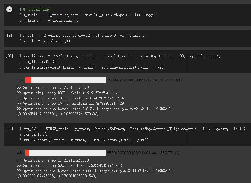
1. Used dual SVM

2. Did not consider regularization, a.k.a. set \(C=\infty\), because this problem (binary classification between 0/9) should be separable, and the representation of \(b\) becomes nasty with regularization.

3. Used the SMO (sequential minimal optimization) algorithm. During optimization, within each iteration, randomly select \(\alpha_1, \alpha_2\), optimize the QP w.r.t. \(\alpha_2\) and update \(\alpha_1\) accordingly. Added constraint \(\alpha_2 \geq 0\) to the \(\alpha_2\) optimizer. This does not constrain \(\alpha_1\geq 0\) directly. However, with the randomization within each iteration, \(\alpha_i \geq 0\) is satisfied when the whole optimzation over \(\alpha\) finally converges.

4. Provide 2 options: Linear Kernel (baseline SVM) or Softmax kernel

   \[K_{SM}(x, y) = \exp{x^\top y}\]

   To avoid explosion on scale, normalized the input \(x\).

   Included the trigonometric feature map \(\phi(x)\) of the softmax kernel for calculating \(b\), (not for \(w\) because when making prediction, we use kernel function instead of \(w^\top \phi\)).

   Use exact kernel instead of approximating kernel with random feature map, because softmax's dimensionality is infinite. Directly compute the exponential in numpy is more efficient.

   The prediction comes like this (vectorized version):

   \[y_{new} = K(X_{new}, X)\cdot (\alpha * y) + b\]

   Note that b is broadcasted to \(n'\) new data points. \(K(X_{new}, X)\) is \(n' \times n\) kernel matrix. \(\alpha*y\) means the elementwise product of two vectors.

5. SVM is expensive when \(n\) is large. Here in practice, we trained on a small batch (default=64). The randomness here influences the performance.

6. Have a few trial runs to get the model with best prediction on the training data. Then it should give good prediction on the validation data. You might also need to tune the hyperparameters a little bit, like batch_size and tol.

Functional/Geometric Margin

两者区别在于 \(w\) 是否被标准化。效用边际会受到参数scale的影响。如果标准化了则两者等效。

Optimal Margin Classifier (Primal)

经过转换，问题变为一个QP问题，可以用一般优化器优化。

Primal:

实现效果

Kernel_FeatureMaps.py

1
2
3
4
5
6
7
8
9
10
11
12
13
14
15
16
17
18
19
20
21
22
23
24
25
26
27
28
29
30
31
32
33
34
35
36
37
38
39
40
41
42
43
44
45
46
47
48
49
50
51
52
53
54
55
56
57
58
59
60
61
62
63
64
65
66
67
68
69
70
71
72
73
74
75
76
77
78
79
80
81
82
83
84
85
86
87
88
89
90

import numpy as np


def gram_schmidt_columns(X):
    Q, R = np.linalg.qr(X)
    return Q


def orthgonalize(V):
    N = V.shape[0]
    d = V.shape[1]
    turns = int(N / d)
    remainder = N % d

    V_ = np.zeros_like(V)

    for i in range(turns):
        v = gram_schmidt_columns(V[i * d:(i + 1) * d, :].T).T
        V_[i * d:(i + 1) * d, :] = v
    if remainder != 0:
        V_[turns * d:, :] = gram_schmidt_columns(V[turns * d:, :].T).T

    return V_


# Generate orthogonal normal weights (w1, ..., wm)
def generateGMatrix(m, d) -> np.array:
    G = np.random.normal(0, 1, (m, d))
    # Renormalize
    norms = np.linalg.norm(G, axis=1).reshape([m, 1])
    return orthgonalize(G) * norms


# Softmax trignometric feature map Φ(x)
def baseline_SM(x, G):
    """Calculate the result of softmax trigonometrix random feature mapping
        Parameters
        ----------
        x: array, dimension = n*d
            Input to the baseline mapping
            Required to be of norm 1 for i=1,...n
        
        G: matrix, dimension = m*d
            The matrix in the baseline random feature mapping
    """
    m = G.shape[0]
    left = np.cos(np.dot(x, G.T).astype(np.float32))
    right = np.sin(np.dot(x, G.T).astype(np.float32))
    return np.exp(0.5) * ((1 / m)**0.5) * np.hstack([left, right])


class Kernel(object):
    """Kernels.
        Parameters
        ---------
        x, y: array of (n_x, d), (n_y, d)
        Return
        ---------
        K(x,y): kernel matrix of (n_x, n_y), K_ij = K(x_i, y_j)
    """
    @staticmethod
    def Linear(x, y):
        return np.dot(x, y.T)

    @staticmethod
    def Softmax(x, y):
        return np.exp(np.dot(x, y.T))


class FeatureMap(object):
    """Feature mapping
    
        Parameters
        ---------
        x: array of (n, d)
        Return
        ---------
        Φ(x): array of (n, m), where m is usually a higher dimensionality. Here we set m = 2*n
    """
    @staticmethod
    def Linear(x):
        return x

    @staticmethod
    def Softmax_Trigonometric(x):
        n, d = x.shape
        # Increase dimensionality to 2x
        G = generateGMatrix(2 * d, d)
        phi_x = baseline_SM(x, G)
        return phi_x

SVM.py

Recap

KKT, Lagrangian

\[L(w, b, \alpha, \beta) = f(w,b) + \sum_{i=1}^{N}{\alpha_ig_i(w,b)} + \sum_{i=1}^{N}{\beta_ih_i(w,b)}\]

\[\theta(w,b) = \max_{\alpha, \beta} L(w, b, \alpha, \beta) \]

\[\theta(w,b) = \begin{cases} f(w,b) \text{\: if feasible} \\ \infty \text{\: otherwise} \end{cases}\]

HW2

Hua Yao, UNI:hy2632

Problem 1: Convolutional Neural Networks [20 points]

The input RGB- image has 3 channels. Apply Conv2D to each channel to get 3 feature maps.

When there's no padding, the shape of 3 feature maps are \(125\times125\).