Code Repo
https://github.com/hy2632/Efficient-Frontier
References
Brief
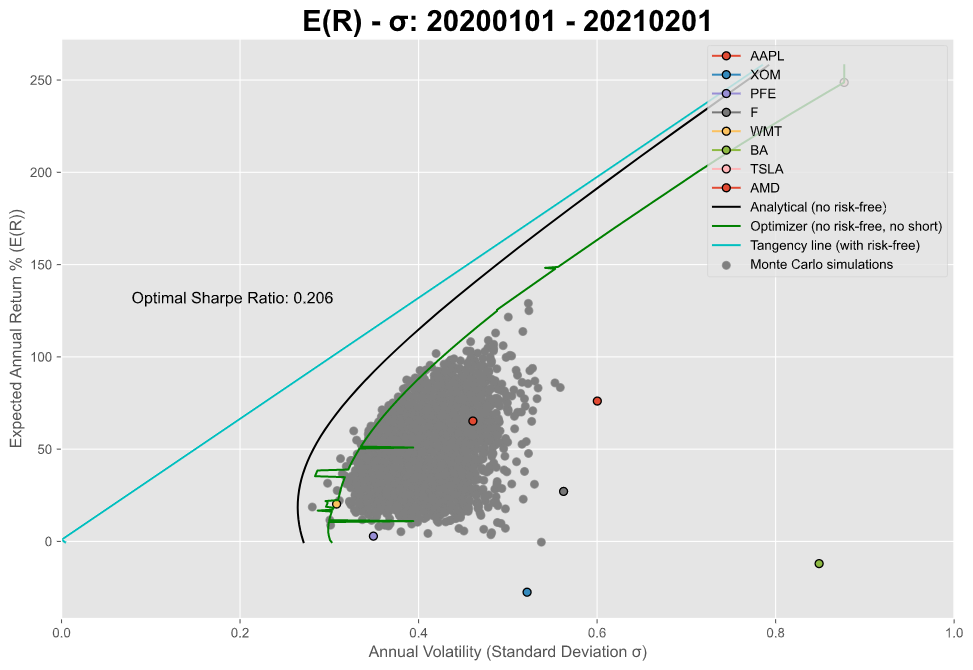
Analysis on the modern portfolio theory.
- Efficient frontier with / without risk free asset
- Optimal sharpe ratio / portfolio
Example of usage
1 | instance = EfficientFrontier( |
Content
- Monte Carlo simulation of portfolios consisting of assets in the designated pool.
- Solve for the curve of the efficient frontier without risk-free asset analytically (a constrained optimization problem) using lagrange multiplier. This solution did not take into consideration the constraint that all weights are greater than 0, a.k.a. it allows short and leverage.
\[ \begin{bmatrix}2\Sigma &-R & -{\bf1}\\ R^T &0 & 0 \\ {\bf1}^T &0 &0 \end{bmatrix} * \begin{bmatrix}w\\\lambda_1\\\lambda_2\end{bmatrix} = \begin{bmatrix}0\\\mu \\ 1\end{bmatrix}\]
(2021/1/30 Update)
optimizerSolver()to solve for the efficient frontier using scipy optimizer. Added the constraint of no short. Due to the limit of the optimizer, this solution performs bad for lowmupart.(2021/2/1 Update)
tangencySolver()which solves for the "with risk-free asset" case. The solution can be proved to be the tangency line of the efficient frontier curve in the "no risk-free asset" setting.Plotting the figure of all above.
2021/2/1: Frontier with risk-free asset —— the tangency line
Consider the constrained problem that
\[ \min{\frac12 w^T\Sigma w} \] \[ \text{s.t. } (1 - \sum_{i=1}^n{w_i})r_f + w^TR = \mu\\ \]
Lagrange multiplier:
\[F = \frac12 w^T\Sigma w - \lambda[w^T(R - r_f {\bf1}) - (\mu - r_f)] \]
\[\frac{\partial F}{\partial w} = \Sigma w - \lambda(R - r_f {\bf1}) = 0 \\ \to w = \lambda \Sigma^{-1} (R - r_f {\bf1})\]
\[ (1 - \sum_{i=1}^n{w_i})r_f + w^TR = \mu \\ \to (R - r_f {\bf1})^T w = \mu - r_f \]
Solution:
\[\therefore \lambda = \frac{\mu - r_f}{(R - r_f {\bf1})^T\Sigma^{-1}(R - r_f {\bf1})} \] \[w = \lambda\Sigma^{-1} (R - r_f {\bf1}) = \frac{(\mu - r_f)\Sigma^{-1} (R - r_f {\bf1})}{(R - r_f {\bf1})^T\Sigma^{-1}(R - r_f {\bf1})}\]
It can be proved that for any combination of risk-free asset and any risky asset, \(\mu / \sigma \propto \alpha\). Therefore, if we got an optimal efficient risky portfolio without risk-free asset, the efficient frontier with risk-free asset should be the tangency line which crosses that point.