Systematic Trading: Early Profit/Loss Taker?

Preface

In Robert Carver's book "Systematic Trading", he compared the two mindsets of trading: "Early Profit Taker" and "Early Loss Taker". The previous one is our mankind's "flawed instinction" and the latter one is believed to outperform the previous one.

This notebook implements the argument and verifies it through different examples.

Some of the parameters in the method is at your own discretion. Stocks and futures might take values to different orders of magnitude w.r.t. the "tolerance_lo", let alone the fact that everyone has his own extent of tolerance.

Import packages and load datasets

1
2
3
4
5
6
7
%cd /content/drive/MyDrive/Quant
import numpy as np
import pandas_datareader as pdr
from pandas_datareader import data
import matplotlib.pyplot as plt
import pandas as pd
import pdb
1
BABA = data.get_data_yahoo("BABA", "20151201", "20201201")
1
2
3
4
5
6
7
8
# Download US 10 Year Treasury Futures dataset from https://www.macrotrends.net/futures/10-year-treasury
USTTEN_Future = pd.read_csv("10-year-treasury-futures.csv", skiprows=16)
USTTEN_Future.rename(columns={" value":"Adj Close"}, inplace=True)
USTTEN_Future["date"] = USTTEN_Future["date"].astype("datetime64")
USTTEN_Future_slice = USTTEN_Future[(USTTEN_Future["date"] > "2011-04-30") & (USTTEN_Future["date"] < "2012-03-01")]

USTTEN_Future_slice.set_index("date", inplace=True)
USTTEN_Future_slice
Adj Close
date
2011-05-02 121.2344
2011-05-03 121.4375
2011-05-04 121.6406
2011-05-05 122.0625
2011-05-06 122.2813
... ...
2012-02-23 131.2031
2012-02-24 131.1344
2012-02-27 131.5125
2012-02-28 131.5031
2012-02-29 131.0156

210 rows × 1 columns

Modeling 2 strategies

1
2
3
4
5
6
7
8
9
10
11
12
13
14
15
16
17
18
19
20
21
22
23
24
25
26
27
28
29
30
31
32
33
34
35
36
37
38
39
40
41
42
43
44
45
46
47
48
49
50
51
52
53
54
55
56
57
58
59
60
61
62
63
64
65
66
67
68
69
70
71
72
def strategy_modeling(
principal = 1e5,
strategy = 'Early_Profit_Taker',
tol_hi = 0.1,
tol_lo = 0.05,
position_hi = 1,
position_lo = 0.1,
data = BABA,
):
"""
This module compare two different transaction strategies: "Early Profit Taker" and "Early Loss Taker", mentioned by Robert Carver
in his book Systematic Trading. The previous one is mankind's instinction, while the latter one usually outperforms.

## Author
Hua Yao (hy2632@columbia.edu)

## Reference:
Robert Carver, Systematic Trading: A unique new method for designing trading and investing systems, Page 15.

Parameters:
---------
principal: int, your principal
strategy: str, 'Early_Profit_Taker' / 'Early_Loss_Taker'
tol_hi: the higher threshold of percentage change in price since last transaction
tol_lo: the lower...
position_hi: high position 高仓位
position_lo: low position 低仓位
data = BABA: pandas_datareader.data.get_data_yahoo style dataframe. Used "Adj Close" as the stock price.

"""


start_date = data.index[0]
end_date = data.index[-1]

last_transaction = 0

position = np.ones(len(data)) * position_hi
num_stocks = np.ones(len(data)) * principal * position_hi / data.iloc[0]["Adj Close"]
book_value = np.ones(len(data)) * principal


if strategy == 'Early_Profit_Taker':
tol_profit = tol_lo
tol_loss = tol_hi
else:
assert strategy == 'Early_Loss_Taker'
tol_profit = tol_hi
tol_loss = tol_lo

for idx in range(1, len(data)):
book_value[idx] = book_value[idx - 1] + num_stocks[idx] * (data.iloc[idx]["Adj Close"] / data.iloc[idx - 1]["Adj Close"] - 1)
if position[idx] == position_lo: # currently in position_lo and last transaction was selling, now buy
if data.iloc[idx]["Adj Close"] / data.iloc[last_transaction]["Adj Close"] - 1 > tol_loss: # the price increases over the tolerance of loss after selling
position[idx + 1:] = position_hi # buy
num_stocks[idx + 1:] = (book_value[idx] * position_hi) / data.iloc[idx]["Adj Close"] # num_stocks decided at buying, high position
last_transaction = idx # record
else:
continue
else: # currently in position_hi and last transaction was buying
if (data.iloc[idx]["Adj Close"] / data.iloc[last_transaction]["Adj Close"] - 1 > tol_profit) | \
(data.iloc[idx]["Adj Close"] / data.iloc[last_transaction]["Adj Close"] - 1 < - tol_loss): # the price increases over the tolerance of profit or decreases over the tolerance of loss after buying
position[idx + 1:] = position_lo # sell out to position_lo
num_stocks[idx + 1:] = (book_value[idx] * position_lo) / data.iloc[idx]["Adj Close"] # num_stocks decided at selling, low position
last_transaction = idx
else:
continue

return position, num_stocks, book_value-principal


Evaluate the performance

1
2
3
4
5
6
7
8
9
10
11
12
13
14
15
16
17
18
19
20
21
22
23
24
25
26
27
28
29
30
31
32
33
34
35
36
37
38
39
40
41
42
43
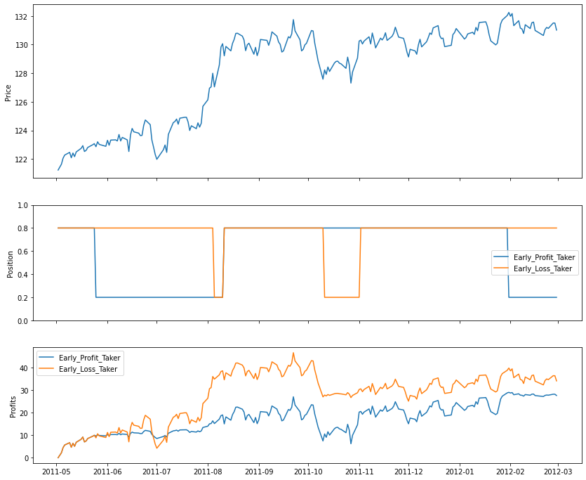
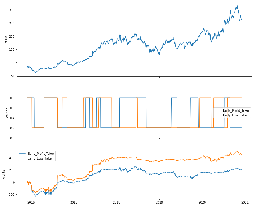
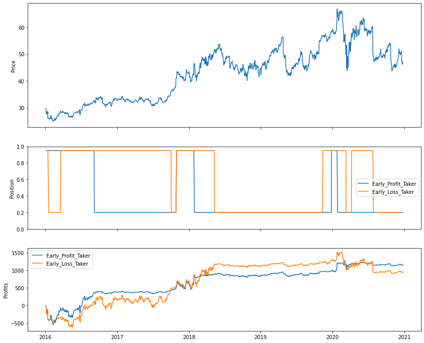
def plot_strategy_comparison(
principal = 1e5,
tol_hi = 0.3,
tol_lo = 0.1,
position_hi = 1,
position_lo = 0.1,
data = BABA,
):

position, num_stocks, gain = strategy_modeling(
principal,
'Early_Profit_Taker',
tol_hi,
tol_lo,
position_hi,
position_lo,
data,
)
position_, num_stocks_, gain_ = strategy_modeling(
principal,
'Early_Loss_Taker',
tol_hi,
tol_lo,
position_hi,
position_lo,
data,
)

# gridspec_kw: https://stackoverflow.com/questions/10388462/matplotlib-different-size-subplots
fig,ax = plt.subplots(3, 1, sharex=True, figsize=(14,12), gridspec_kw={'height_ratios': [3, 2, 2]})
ax[0].plot(data.index, data["Adj Close"])
ax[0].set_ylabel("Price")
ax[1].plot(data.index, position)
ax[1].plot(data.index, position_)
ax[1].set_ylim(0, 1)
ax[1].legend(["Early_Profit_Taker", "Early_Loss_Taker"])
ax[1].set_ylabel("Position")
ax[2].plot(data.index, gain)
ax[2].plot(data.index, gain_)
ax[2].legend(["Early_Profit_Taker", "Early_Loss_Taker"])
ax[2].set_ylabel("Profits")

plt.show()

Example: The US Ten year treasury future (2011.05 - 2012.03)

1
2
3
4
5
6
7
8
plot_strategy_comparison(
principal=1e5,
tol_hi=0.055,
tol_lo=0.015,
position_hi=0.8,
position_lo = 0.2,
data=USTTEN_Future_slice,
)

Example: BABA

1
2
3
4
5
6
7
8
plot_strategy_comparison(
principal=1e5,
tol_hi=0.2,
tol_lo=0.1,
position_hi=0.8,
position_lo = 0.2,
data=BABA,
)

1
2
3
4
5
6
7
8
plot_strategy_comparison(
principal=1e5,
tol_hi=0.25,
tol_lo=0.1,
position_hi=0.95,
position_lo = 0.2,
data=data.get_data_yahoo("INTC", "20160101", "20201224"),
)

Comment

The values of tol_hi and tol_lo as well as the ratio between them, are hard to be determined, and collectively influences the payoff. The conditions where the argument holds remain unclear.