Data-Mining-HW1

Description

1 Problem 1: Softmax-kernel approximators [50 points]

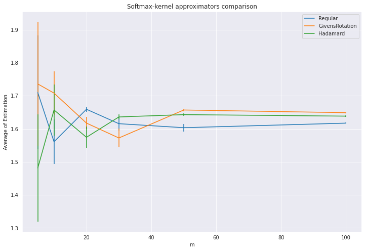
The goal of this task is to test different random feature map based estimators of the softmax-kernel. Choose two feature vectors \(x, y \in \mathbb{R}^{20}\) of unit \(L_2\)-norm and with angle \(\frac{π}{3}\) between them. Consider three estimators of the value of the softmax-kernel in these points: the regular one using independent sin/cos-random features (leveraging random feature maps for the Gaussian kernel) and its two modifications: the one using Givens random rotations and the one applying random Hadamard matrices (with three HD-blocks). Describe in detail each estimator. Then for the number of random projections \(m = 5, 10, 20, 30, 50, 100\) and each estimator, compute its value as an average over \(s = 10\) independent trials. Propose how to use those trials to compute empirical mean squared error for each estimator. Prepare plots where on \(x\)-axis you put the number of random projections m used and on the \(y\)-axis the average value of the estimator. Show also computed mean squared error in the form of the error-bars. Remark: If \(m > d\) the orthogonal trick can be still applied by constructing independent ensembles of samples such that within each ensemble samples are exactly orthogonal.

Problem 2 Softmax-kernel is positive semidefinite [30 points]

\(K : \mathbb{R}^{d\times d} \to \mathbb{R}^{d}\) is positive semidefinite (PSD) if:

\[v^T\kappa(X)v \geq 0\]

for any \(N>0\), any set of feature vectors \(\chi = \{x_1, ..., x_N\}\subseteq \mathbb{R}^d\), matrix \(\kappa(X) := [K(x_i, x_j)]_{i,j=1,...,N} \in \mathbb{R}^{N\times N}\) and any vector \(v \in \mathbb{R}^{N}\). Show that softmax-kernel is PSD.

Proof:

\[X \in \mathbb{R}^{d\times N},\] \[\kappa(X)_{ij} = K_{SM}(x_i, x_j) = e^{x_i^Tx_j}\] \[ \kappa(X) = \exp{(X^TX)} \in \mathbb{R}^{N\times N}\]

Lemma1: \(X^TX \in \mathbb{R}^N and \ XX^T \in \mathbb{R}^d\) are PSD

Proof:

\[v^T(X^TX)v = (Xv)^T(Xv) = y^Ty \geq 0\]

\[v \in \mathbb{R}^{N}\]

\[y = Xv \in \mathbb{R}^{d}\]

Similarly, $XX^T $ is PSD

Lemma2: \((X^TX)^k \ and \ (XX^T)^k, k=0,1,2,...\) are PSD.

Proof:

For \(k=0\), obviously \(I\) is PSD.

From above, this holds when \(k=1\). Use mathematical induction, if this is true for \(k=n-1\), then for \(k=n\) \[ v^T(X^TX)^{n}v = (Xv)^T(XX^T)^{n-1}(Xv) = y^T(XX^T)^{n-1}y \geq 0\] \[ v\in \mathbb{R}^N, y = Xv \in \mathbb{R}^d\] \[ u^T(XX^T)^{n}u = (X^Tu)^T(X^TX)^{n-1}(X^Tu) = z^T(X^TX)^{n-1}z \geq 0,\ z\in \mathbb{R}^N \] \[ u\in \mathbb{R}^d, z=X^Tu\in \mathbb{R}^N\]

Therefore this holds for arbitrary \(k \in \{0,1,2,3...\}\).

Lemma3: Matrix exponential

The exponential of a \(N\times N\) matrix \(X\) is: \[e^{X} = \sum_{k=0}^{\infty}{\frac{1}{k!}X^k}\]

Using results above,

\[ \therefore \kappa(X) = \exp{(X^TX)} = \sum_{k=0}^{\infty}{\frac{1}{k!}(X^TX)^k}\]

\[ v^T\kappa(X)v = \sum_{k=0}^{\infty}{\frac{1}{k!}v^T(X^TX)^kv} \geq 0\]

\(\therefore\) Softmax-kernel is PSD.

Notebook for Problem 1

Import packages

import numpy as np
import math
from sklearn.metrics import mean_squared_error 
import matplotlib.pyplot as plt
import os
import random
import pandas as pd
import seaborn as sns
from tqdm import tqdm
import datetime
from scipy.stats import norm
from scipy.spatial.transform import Rotation as R
import scipy as sp

Problem 1: Softmax-kernel approximators [50 points]

Choose two feature vectors \(x, y \in \mathbb{R}^{20}\) of unit \(L_2\)-norm and with angle \(\frac{π}{3}\) between them.

def generateXY(d = 20):
    # init X
    x = np.array([1] + [0]*(d-1))
    y = np.array([0.5, 3**0.5/2] + [0]*(d-2))

    # Orthogonal Matrix Q
    A = np.random.normal(0, 1, (d,d))
    Q, _ = np.linalg.qr(A, mode = 'complete')

    # x^Ty=0.5 => (Qx)^T(Qy)=0.5, where Q is orthogonal
    x = np.matmul(Q, x)
    y = np.matmul(Q, y)
    return x,y
    

x, y = generateXY(20)
x, y

(array([-0.29894506, -0.66638541, -0.18786531, -0.08032163,  0.01395138,
         0.002299  ,  0.1465464 ,  0.32123403, -0.13995845,  0.17208692,
        -0.30362139, -0.20299325, -0.00676445, -0.17788199, -0.00389046,
         0.11739096,  0.13262346, -0.07173246,  0.18018864, -0.12911171]),
 array([ 0.05091238, -0.50959723,  0.39335244, -0.36683427,  0.11539508,
        -0.07330203,  0.07384118,  0.13288575, -0.47794303,  0.09279718,
        -0.08177025,  0.01269871, -0.01592124,  0.1074321 , -0.0916396 ,
         0.05875871,  0.19641505, -0.27930029,  0.14967152,  0.01007921]))

\(K_{SM}(x,y) = e^{x^Ty} = e^{0.5}\)

true_value = np.exp(np.dot(x, y))
true_value

1.6487212707001284

Consider three estimators of the value of the softmax-kernel in these points; Describe in detail each estimator.

• the regular one using independent sin/cos-random features (leveraging random feature maps for the Gaussian kernel)
• and its two modifications: the one using Givens random rotations
• and the one applying random Hadamard matrices (with three HD-blocks).

Answer

• Regular one:
  • Generate matrix \(G:N(0,I_d) \in \mathbb{R}^{m\times d}\)
  • caculate the norms of each row(\(|w_i|^2\sim \chi^2(d)\))
  • Map through \(G\)'s \(m\) rows and orthogonalize \(G\)'s each \(d\times d\) block(or the remainder part \((m\%d) \times d\))
  • Renormalize the orthogonalized matrix with its original row norms. \[ \phi_{SM}(x) = e^{\frac{||x||^2}{2}} \frac{1}{\sqrt{m}} \begin{bmatrix}\cos(w_1^Tx)\\...\\\cos(w_m^Tx)\\\sin(w_1^Tx)\\...\\\sin(w_m^Tx) \end{bmatrix} \]
  • Calculate \(\phi(x)\) and \(\phi(y)\), and thus \(\phi(x)^T\phi(y)\)
• Givens random rotations:
  • Generate random Givens Matrices \(\{Giv_i \in \mathbb{R}^{d\times d}\}, i=1,...,k = d\log{d}\)
  • Generate orthogonal \(d\times d\) matrix \(G_{ort} = Giv_1,...Giv_k\)
  • Generate diagnoal matrix \(S\) with entries \(S_{ii}\) such that \(S_{ii} \sim \chi(d)\)
  • Renormalize \(G_{ort}\) by left multiplying \(S\)
  • Generate several such \(G_{ort} \in \mathbb{R}^{d\times d}\) and concatenate to get \(G_{ort} \in \mathbb{R}^{m\times d}\)
  • Apply the softmax random feature function \(\phi_{SM}\) like the regular one
• Hadamard Matrices
  • Calculate the padded size \(d' = 2^T\)
  • Pad the input \(x\) and \(y\) to dimension of \(d'\)
  • Generate Hadamard Matrix \(H: d' \times d'\)
  • Generate 3 random diagonal "sign-flipping" matrices \(D_i\)
  • Generate diagnoal matrix \(S\) with entries \(S_{ii}\) such that \(S_{ii} \sim \chi(d')\)
  • \(G_{ort} = S(\frac{1}{\sqrt{d'}}HD_1)(\frac{1}{\sqrt{d'}}HD_2)(\frac{1}{\sqrt{d'}}HD_3)\)
  • Generate several such \(G_{ort} \in \mathbb{R}^{d'\times d'}\) and concatenate to get \(G_{ort} \in \mathbb{R}^{m\times d'}\)
  • Apply the softmax random feature function \(\phi_{SM}\) like the regular one

Then for the number of random projections \(m = 5, 10, 20, 30, 50, 100\) and each estimator, compute its value as an average over \(s = 10\) independent trials.

Estimator1: Regular one

\[ \phi_{SM}(x) = e^{\frac{||x||^2}{2}}\phi_{Gauss}(x) = e^{\frac{||x||^2}{2}} \frac{1}{\sqrt{m}} \begin{bmatrix}\cos(w_1^Tx)\\...\\\cos(w_m^Tx)\\\sin(w_1^Tx)\\...\\\sin(w_m^Tx) \end{bmatrix} \]

def gram_schmidt_columns(X):
    Q, R = np.linalg.qr(X)
    return Q

def orthgonalize(V):
    N = V.shape[0]
    d = V.shape[1]
    turns = int(N/d)
    remainder = N%d
    
    #V =  np.random.normal(size=[(turns+1)*d, d])
    #V =  np.random.normal(size =[N, d])
    #print(V.shape)
    V_ = np.zeros_like(V)
    
    for i in range(turns):
        v = gram_schmidt_columns(V[i*d:(i+1)*d, :].T).T
        V_[i*d:(i+1)*d, :] = v
    if remainder != 0:
        V_[turns*d:,:] = gram_schmidt_columns(V[turns*d:,:].T).T
        
    return V_
    
def generateGMatrix(m = 5, d = 20) -> np.array:
    G = np.random.normal(0,1, (m,d))
    # Renormalize
    norms = np.linalg.norm(G, axis=1).reshape([m,1])
    return orthgonalize(G) * norms

# Softmax with sin/cos random features
def baseline_SM(x, G, m):
    """Calculate the result of baseline random feature mapping

        Parameters
        ----------
        x: array, dimension = d
            The data point to input to the baseline mapping
        
        G: matrix, dimension = m*d
            The matrix in the baseline random feature mapping
            
        m: integer
            The number of dimension that we want to reduce to
    """
    left = np.cos(np.dot(G, x).astype(np.float32))
    right = np.sin(np.dot(G, x).astype(np.float32))
    return np.exp( (np.linalg.norm(x))**2 / 2) * ((1/m)**0.5) * np.append(left, right)

def baseline_SM_approximation(x, y, m, d=20, s=10):
    sum = 0
    for i in range(s):
        G = generateGMatrix(m=m, d=d)
        phi_x = baseline_SM(x, G, m)
        phi_y = baseline_SM(y, G, m)
        xTy = np.dot(phi_x, phi_y)
        sum += xTy
    return sum / s

arr_m = [5, 10, 20, 30, 50, 100]
arr_estimation = [baseline_SM_approximation(x, y, i, 20, 10) for i in arr_m]
arr_estimation

[1.8072113811969757,
 1.69626122713089,
 1.6249037623405456,
 1.670891809463501,
 1.6728131294250488,
 1.640375828742981]

Estimator2: Givens random rotations

\(G_{ort} = Giv_1,...Giv_k, k=O(d\log{d})\)

\(Giv_i \in \mathbb{R}^{d\times d}\)

Orthogonal Random Features

The idea of Orthogonal Random Features (ORF) is to impose orthogonality on the matrix on the linear transformation matrix \(G\). Note that one cannot achieve unbiased kernel estimation by simply replacing \(G\) by an orthogonal matrix, since the norms of the rows of \(G\) follow the -distribution, while rows of an orthogonal matrix have the unit norm. The linear transformation matrix of ORF has the following form \[W_{ORF} = \frac{1}{\sigma} SQ\] where \(Q\) is a uniformly distributed random orthogonal matrix. The set of rows of \(Q\) forms a bases in \(R^d\). \(S\) is a diagonal matrix, with diagonal entries sampled i.i.d. from the \(\chi\)-distribution

def generateGiv(d):
    Giv = np.identity(d)
    i = np.random.randint(0, d-1)
    j = np.random.randint(i+1, d)
    theta = np.random.uniform(0, 2*np.pi)
    c = np.cos(theta)
    s = np.sin(theta)
    Giv[i,i] = c
    Giv[j,j] = c
    Giv[i,j] = s
    Giv[j, i] = -s
    return Giv

def generateS(d):
    return np.diag(np.sqrt(np.random.chisquare(d, (d))))

def Givens_generateGort_dd(d):
    k = int(d * np.log(d))
    Gort_dd = generateGiv(d)
    for i in range(k-1):
        Gort_dd = np.matmul(Gort_dd, generateGiv(d))
    return np.matmul(generateS(d), Gort_dd)

def Givens_generateGort_md(m, d):
    arr_Gort_dd = []
    for i in range(m//d + 1):
        arr_Gort_dd.append(Givens_generateGort_dd(d)) # (m//d+1, d, d)
    Gort_md = np.concatenate(arr_Gort_dd, axis=0)
    Gort_md = Gort_md[:m, :]

    return Gort_md

def GivensRandomRotations_SM_approximation(x, y, m, d=20, s=10):
    sum = 0
    for i in range(s):
        G = Givens_generateGort_md(m,20)
        phi_x = baseline_SM(x, G, m)
        phi_y = baseline_SM(y, G, m)
        xTy = np.dot(phi_x, phi_y)
        sum += xTy
    return sum / s

arr_m = [5, 10, 20, 30, 50, 100]
arr_estimation = [GivensRandomRotations_SM_approximation(x, y, i, 20, 10) for i in arr_m]
arr_estimation

[1.3707373946905137,
 1.7438804149627685,
 1.6728084802627563,
 1.7161020755767822,
 1.689209222793579,
 1.6569807291030885]

Estimator3: Hadamard matrices(with 3 HD-blocks)

def Hadamard(d):
    """return: Hadamard matrix of shape(2^d, 2^d)
    """
    if d==0:
        return np.ones((1,1))
    else:
        ul = Hadamard(d-1)
        ur = Hadamard(d-1)
        bl = Hadamard(d-1)
        br = -Hadamard(d-1)
        u = np.concatenate((ul,ur),axis=1)
        b = np.concatenate((bl,br),axis=1)
        return np.concatenate((u,b),axis=0)

def normalized_Hadamard(d):
    H = Hadamard(d)
    norms = np.linalg.norm(H, axis=1)
    return H / norms
    

def generateDi(d):
    D_i = np.diag([np.random.choice([1, -1]) for i in range(1, d+1)])
    return D_i

# Uncomment to get Structured Orthogonal Random Features (SORF) solution

def Hadamard_generateGort_dd(d): 
    t = np.ceil(np.log2(d)).astype(int)
    d_ = 2**t
    # H = normalized_Hadamard(t)
    H = Hadamard(t)
    Gort_dd = np.identity(d_)
    for i in range(3):
        # Gort_dd = np.matmul(Gort_dd ,np.matmul(H, generateDi(d_)))
        Gort_dd = np.matmul(Gort_dd ,np.matmul(1 / np.sqrt(d_) * H, generateDi(d_)))
    # return np.sqrt(d_)*Gort_dd
    return np.matmul(generateS(d_), Gort_dd)

def Hadamard_generateGort_md(m, d):
    t = np.floor(np.log2(d)).astype(int) + 1
    d_ = 2**t
    arr_Gort_dd = []
    for i in range(m//d_ + 1):
        arr_Gort_dd.append(Hadamard_generateGort_dd(d))
    Gort_md = np.concatenate(arr_Gort_dd, axis=0)
    Gort_md = Gort_md[:m, :]

    return Gort_md

def Hadamard_SM_approximation(x, y, m, d=20, s=10):
    sum = 0
    for i in range(s):
        G = Hadamard_generateGort_md(m,20)
        d_ = G.shape[1]
        x_padded = np.pad(x, (0, d_-d))
        y_padded = np.pad(y, (0, d_-d))
        phi_x = baseline_SM(x_padded, G, m)
        phi_y = baseline_SM(y_padded, G, m)
        xTy = np.dot(phi_x, phi_y)
        sum += xTy
    return sum / s

arr_m = [5, 10, 20, 30, 50, 100]
arr_estimation = [Hadamard_SM_approximation(x, y, i, 20, 10) for i in arr_m]
arr_estimation

[1.7086819410324097,
 1.617677903175354,
 1.6517545461654664,
 1.645971429347992,
 1.6519848704338074,
 1.6540889978408813]

Propose how to use those trials to compute empirical mean squared error for each estimator.

Answer

• The true value: \(K_{SM}(x,y) = e^{x^Ty} = e^{0.5}\)
• For each \(m\), run 10 trials. \[MSE = \frac{\sum_{i=1}^{10}{(est_i - e^{0.5}})^2}{10}\]

def MSE_iid(
    SM_approximation=Hadamard_SM_approximation,
    episode=1, 
    epoch=10, 
    arr_m=[5, 10, 20, 30, 50, 100],
    ):

    estimation = np.zeros((len(arr_m), episode, epoch))
    MSE_iid = []
    list_of_samples = []

    x, y = generateXY(20)

    # for e in tqdm(range(episode), position=0, leave=True):
    #     x, y = generateXY(20)
    #     true_value = np.exp(0.5)
    #     list_of_samples.append((x, y))

    for n in range(len(arr_m)):
        mse_m = []
        m = arr_m[n]
        
        for e in tqdm(range(episode), position=0, leave=True):        
            # x = list_of_samples[e][0]
            # y = list_of_samples[e][1]
            for i in range(epoch):
                np.random.seed()
                estimation[n, e, i] = SM_approximation(x, y, m, d=20, s=1)

            mse_m.append(mean_squared_error(np.repeat(true_value, epoch), estimation[n, e])) # compare 10 values
        
        MSE_iid.append(mse_m)
    
    return estimation.mean(axis=(1,2)) ,MSE_iid

estimation_regular, MSE_iid_regular = MSE_iid(SM_approximation=baseline_SM_approximation)
df_MSE_Regular = pd.DataFrame(MSE_iid_regular, index = arr_m, columns = ["Regular"])
df_estimation_Regular = pd.DataFrame(estimation_regular, index = arr_m, columns = ["Regular"])

100%|██████████| 1/1 [00:00<00:00, 101.45it/s]
100%|██████████| 1/1 [00:00<00:00, 119.49it/s]
100%|██████████| 1/1 [00:00<00:00, 95.60it/s]
100%|██████████| 1/1 [00:00<00:00, 112.89it/s]
100%|██████████| 1/1 [00:00<00:00, 89.43it/s]
100%|██████████| 1/1 [00:00<00:00, 74.54it/s]

estimation_Givens, MSE_iid_Givens = MSE_iid(SM_approximation=GivensRandomRotations_SM_approximation)
df_MSE_Givens = pd.DataFrame(MSE_iid_Givens, index = arr_m, columns = ["GivensRotation"])
df_estimation_Givens = pd.DataFrame(estimation_Givens, index = arr_m, columns = ["GivensRotation"])

100%|██████████| 1/1 [00:00<00:00, 25.62it/s]
100%|██████████| 1/1 [00:00<00:00, 30.17it/s]
100%|██████████| 1/1 [00:00<00:00, 13.01it/s]
100%|██████████| 1/1 [00:00<00:00, 16.68it/s]
100%|██████████| 1/1 [00:00<00:00, 14.39it/s]
100%|██████████| 1/1 [00:00<00:00,  6.19it/s]

estimation_Hadamard, MSE_iid_Hadamard = MSE_iid(SM_approximation=Hadamard_SM_approximation)
df_MSE_Hadamard = pd.DataFrame(MSE_iid_Hadamard, index = arr_m, columns = ["Hadamard"])
df_estimation_Hadamard = pd.DataFrame(estimation_Hadamard, index = arr_m, columns = ["Hadamard"])

100%|██████████| 1/1 [00:00<00:00, 12.08it/s]
100%|██████████| 1/1 [00:00<00:00, 11.96it/s]
100%|██████████| 1/1 [00:00<00:00, 12.45it/s]
100%|██████████| 1/1 [00:00<00:00, 12.02it/s]
100%|██████████| 1/1 [00:00<00:00,  7.46it/s]
100%|██████████| 1/1 [00:00<00:00,  3.86it/s]

df_MSE_total = pd.concat([df_MSE_Regular, df_MSE_Givens, df_MSE_Hadamard], axis=1)
df_estimation_total = pd.concat([df_estimation_Regular, df_estimation_Givens, df_estimation_Hadamard], axis=1)

df_MSE_total

	Regular	GivensRotation	Hadamard
5	0.172311	0.188588	0.162290
10	0.066876	0.065423	0.077146
20	0.007488	0.017989	0.032074
30	0.020978	0.027808	0.007083
50	0.011074	0.003390	0.004394
100	0.001614	0.001725	0.001746

df_estimation_total

	Regular	GivensRotation	Hadamard
5	1.709679	1.735700	1.481327
10	1.560758	1.708040	1.657001
20	1.659077	1.617314	1.574311
30	1.615470	1.572253	1.635823
50	1.603345	1.656838	1.642844
100	1.617124	1.648726	1.638272

Prepare plots where on x-axis you put the number of random projections m used and on the y-axis the average value of the estimator. Show also computed mean squared error in the form of the error-bars

sns.set_style("darkgrid")    
df_estimation_total.plot(
    kind = 'line', 
    title = 'Softmax-kernel approximators comparison', 
    grid=True, 
    legend=[df_estimation_total.columns],
    xlabel='m', 
    ylabel='Average of Estimation',
    figsize = (12,8),
    yerr=df_MSE_total,
    )
plt.show()